参考项目:naklecha/llama3-from-scratch 、图解llama架构 解读源码实现
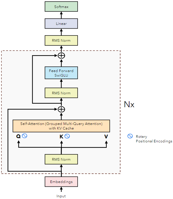
完整结构:Llama 内部结构拆解
1 准备工作 1.1 创建虚拟环境 1 2 3 4 5 conda create -n llama3 python=3.10 list
1.2 下载模型文件 1 huggingface-cli download meta-llama/Meta-Llama-3-8B --include "original/*" --token Your_token --local-dir model/Llama-3-8B
1.3 创建分词器 使用 BPE 分词器,来自 karpathy/minbpe :
1 2 3 4 5 6 7 8 9 10 11 12 13 14 15 16 17 18 19 20 21 22 23 24 25 26 27 28 29 30 31 32 33 34 from pathlib import Pathimport tiktokenfrom tiktoken.load import load_tiktoken_bpeimport torchimport jsonimport matplotlib.pyplot as plt"../model/Llama-3-8B/original/tokenizer.model" "<|begin_of_text|>" ,"<|end_of_text|>" ,"<|reserved_special_token_0|>" ,"<|reserved_special_token_1|>" ,"<|reserved_special_token_2|>" ,"<|reserved_special_token_3|>" ,"<|start_header_id|>" ,"<|end_header_id|>" ,"<|reserved_special_token_4|>" ,"<|eot_id|>" , f"<|reserved_special_token_{i} |>" for i in range (5 , 256 - 5 )]r"(?i:'s|'t|'re|'ve|'m|'ll|'d)|[^\r\n\p{L}\p{N}]?\p{L}+|\p{N}{1,3}| ?[^\s\p{L}\p{N}]+[\r\n]*|\s*[\r\n]+|\s+(?!\S)|\s+" , len (mergeable_ranks) + i for i, token in enumerate (special_tokens)}, "hello world!" ))
'hello world!'
1.4 加载模型参数
加载模型权重:
1 2 model = torch.load("../model/Llama-3-8B/original/consolidated.00.pth" )print (json.dumps(list (model.keys())[:20 ], indent=4 ))
[
"tok_embeddings.weight",
"layers.0.attention.wq.weight",
"layers.0.attention.wk.weight",
"layers.0.attention.wv.weight",
"layers.0.attention.wo.weight",
"layers.0.feed_forward.w1.weight",
"layers.0.feed_forward.w3.weight",
"layers.0.feed_forward.w2.weight",
"layers.0.attention_norm.weight",
"layers.0.ffn_norm.weight",
"layers.1.attention.wq.weight",
"layers.1.attention.wk.weight",
"layers.1.attention.wv.weight",
"layers.1.attention.wo.weight",
"layers.1.feed_forward.w1.weight",
"layers.1.feed_forward.w3.weight",
"layers.1.feed_forward.w2.weight",
"layers.1.attention_norm.weight",
"layers.1.ffn_norm.weight",
"layers.2.attention.wq.weight"
]
加载配置文件:
1 2 3 with open ("../model/Llama-3-8B/original/params.json" , "r" ) as f:
{'dim': 4096,
'n_layers': 32,
'n_heads': 32,
'n_kv_heads': 8,
'vocab_size': 128256,
'multiple_of': 1024,
'ffn_dim_multiplier': 1.3,
'norm_eps': 1e-05,
'rope_theta': 500000.0}
定义模型参数:
1 2 3 4 5 6 7 8 9 dim = config["dim" ] "n_layers" ] "n_heads" ] "n_kv_heads" ] "vocab_size" ] "multiple_of" ] "ffn_dim_multiplier" ] "norm_eps" ] "rope_theta" ])
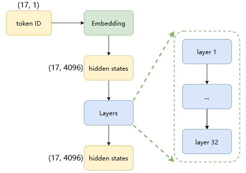
2 分词
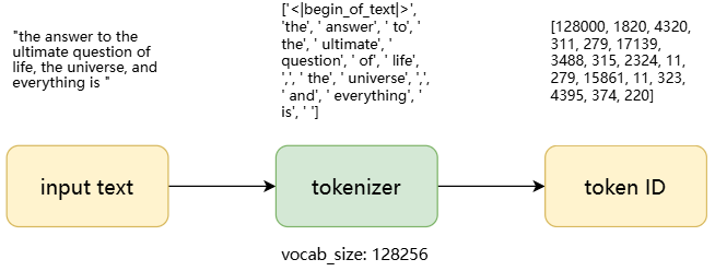
将输入的文本通过分词器变成 token ID:
1 2 3 4 5 6 7 8 9 prompt = "the answer to the ultimate question of life, the universe, and everything is " 128000 ] + tokenizer.encode(prompt)print (tokens)for token in tokens]print (prompt_split_as_tokens)
[128000, 1820, 4320, 311, 279, 17139, 3488, 315, 2324, 11, 279, 15861, 11, 323, 4395, 374, 220]
['<|begin_of_text|>', 'the', ' answer', ' to', ' the', ' ultimate', ' question', ' of', ' life', ',', ' the', ' universe', ',', ' and', ' everything', ' is', ' ']
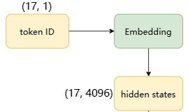
将 17 个 token ID 转换成 17 个 token embedding:
1 2 3 4 embedding_layer = torch.nn.Embedding(vocab_size, dim)"tok_embeddings.weight" ])
torch.Size([17, 4096])
3 RMSNorm 这种归一化的方法可以在保持精度的情况下最大化计算效率,张量形状不变,过程如下:
计算输入张量每个元素的平方。
对平方后的张量沿着最后一个维度计算均值,并保持维度不变,这样得到每个元素的均方值。
将均方值加上一个很小的正数(避免除以零),然后计算其平方根的倒数,得到 RMS 的倒数。
将输入张量与 RMS 的倒数相乘,再乘以归一化权重,得到归一化后的张量。
1 2 3 4 5 def rms_norm (tensor, norm_weights ):return (tensor * torch.rsqrt(tensor.pow (2 ).mean(-1 , keepdim=True ) + norm_eps)) * norm_weights
对 17 个 token embedding 归一化:
1 2 token_embeddings = rms_norm(token_embeddings_unnormalized, model["layers.0.attention_norm.weight" ])
torch.Size([17, 4096])
4 注意力头:以第一层为例 查看第一层所有注意力头的权重矩阵:
1 2 3 4 5 6 print ("layers.0.attention.wq.weight" ].shape, "layers.0.attention.wk.weight" ].shape, "layers.0.attention.wv.weight" ].shape, "layers.0.attention.wo.weight" ].shape
torch.Size([4096, 4096]) torch.Size([1024, 4096]) torch.Size([1024, 4096]) torch.Size([4096, 4096])
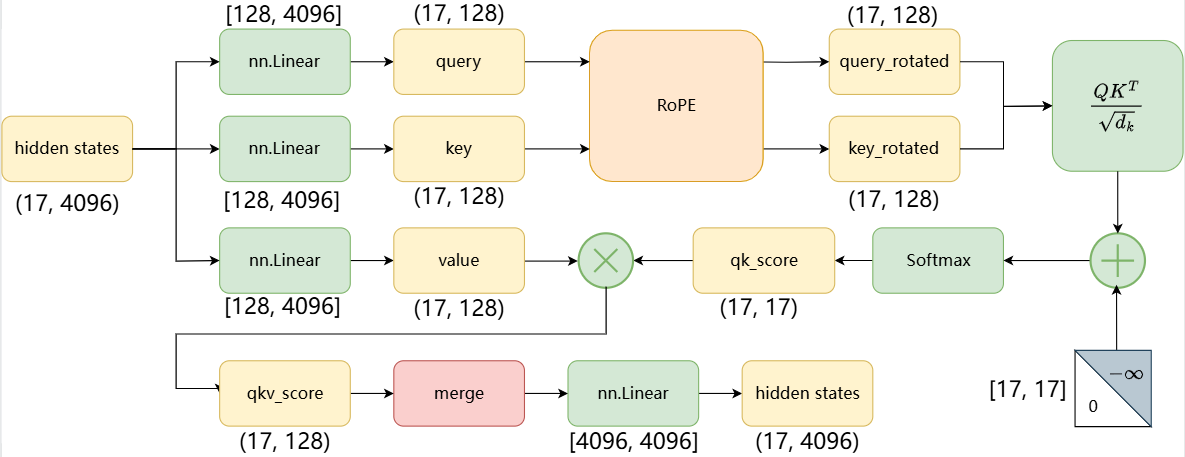
4.1 单头注意力:以第一层的第一个注意力头为例 4.1.1 query
查看第一层所有注意力头的 query 的权重矩阵:
1 2 3 4 q_layer0 = model["layers.0.attention.wq.weight" ]0 ] // n_heads
torch.Size([32, 128, 4096])
查看第一层第一个注意力头的 query 的权重矩阵:
1 2 q_layer0_head0 = q_layer0[0 ]
torch.Size([128, 4096])
将第一层第一个注意力头的 query 权重矩阵与 token embedding 相乘,得到每个 token 的 query:
1 2 q_per_token = torch.matmul(token_embeddings, q_layer0_head0.T)
torch.Size([17, 128])
4.1.2 key key 和 query 的计算流程一致,不过其权重矩阵只有 query 权重矩阵的 1/4,因为 key 的权重矩阵在 4 个头之间共享,以减少所需的计算量。
Grouped Multi-Query Attention(分组多查询注意力)是一种 平衡计算效率和模型性能 的注意力变体,介于 Multi-Head Attention (MHA) 和 Multi-Query Attention (MQA) 之间。它通过分组共享 Key/Value 矩阵 来减少计算量,同时保持较强的表达能力。
查看第一层所有注意力头的 key 的权重矩阵:
1 2 3 k_layer0 = model["layers.0.attention.wk.weight" ]0 ] // n_kv_heads, dim)
torch.Size([8, 128, 4096])
查看第一层第一个注意力头的 key 的权重矩阵:
1 2 k_layer0_head0 = k_layer0[0 ]
torch.Size([128, 4096])
将第一层第一个注意力头的 key 的权重矩阵与 token embedding 相乘,得到每个 token 的 key:
1 2 k_per_token = torch.matmul(token_embeddings, k_layer0_head0.T)
torch.Size([17, 128])
4.1.3 value 和 key 一样,value 权重矩阵也在每 4 个注意力头之间进行共享。
KV Cache 用于加速自回归生成,其核心思想是缓存已计算的 key 和 value 矩阵,避免重复计算,从而显著减少推理时的计算量和内存访问开销。
查看第一层所有注意力头的 value 的权重矩阵:
1 2 3 v_layer0 = model["layers.0.attention.wv.weight" ]0 ] // n_kv_heads, dim)
torch.Size([8, 128, 4096])
查看第一层第一个注意力头的 value 的权重矩阵:
1 2 v_layer0_head0 = v_layer0[0 ]
torch.Size([128, 4096])
将第一层第一个注意力头的 value 的权重矩阵与 token embedding 相乘,得到每个 token 的 value:
1 2 v_per_token = torch.matmul(token_embeddings, v_layer0_head0.T)
torch.Size([17, 128])
4.1.4 RoPE(旋转位置编码) 每个 token 都有一个 query 和 key,但是每个 query 和 key 并不知道它们在文本中的位置,因此需要进行位置编码。
创建一个包含 64 个元素的张量:
1 2 zero_to_one_split_into_64_parts = torch.tensor(range (64 ))/64
tensor([0.0000, 0.0156, 0.0312, 0.0469, 0.0625, 0.0781, 0.0938, 0.1094, 0.1250,
0.1406, 0.1562, 0.1719, 0.1875, 0.2031, 0.2188, 0.2344, 0.2500, 0.2656,
0.2812, 0.2969, 0.3125, 0.3281, 0.3438, 0.3594, 0.3750, 0.3906, 0.4062,
0.4219, 0.4375, 0.4531, 0.4688, 0.4844, 0.5000, 0.5156, 0.5312, 0.5469,
0.5625, 0.5781, 0.5938, 0.6094, 0.6250, 0.6406, 0.6562, 0.6719, 0.6875,
0.7031, 0.7188, 0.7344, 0.7500, 0.7656, 0.7812, 0.7969, 0.8125, 0.8281,
0.8438, 0.8594, 0.8750, 0.8906, 0.9062, 0.9219, 0.9375, 0.9531, 0.9688,
0.9844])
计算频率值:
1 2 freqs = 1.0 / (rope_theta ** zero_to_one_split_into_64_parts)
tensor([1.0000e+00, 8.1462e-01, 6.6360e-01, 5.4058e-01, 4.4037e-01, 3.5873e-01,
2.9223e-01, 2.3805e-01, 1.9392e-01, 1.5797e-01, 1.2869e-01, 1.0483e-01,
8.5397e-02, 6.9566e-02, 5.6670e-02, 4.6164e-02, 3.7606e-02, 3.0635e-02,
2.4955e-02, 2.0329e-02, 1.6560e-02, 1.3490e-02, 1.0990e-02, 8.9523e-03,
7.2927e-03, 5.9407e-03, 4.8394e-03, 3.9423e-03, 3.2114e-03, 2.6161e-03,
2.1311e-03, 1.7360e-03, 1.4142e-03, 1.1520e-03, 9.3847e-04, 7.6450e-04,
6.2277e-04, 5.0732e-04, 4.1327e-04, 3.3666e-04, 2.7425e-04, 2.2341e-04,
1.8199e-04, 1.4825e-04, 1.2077e-04, 9.8381e-05, 8.0143e-05, 6.5286e-05,
5.3183e-05, 4.3324e-05, 3.5292e-05, 2.8750e-05, 2.3420e-05, 1.9078e-05,
1.5542e-05, 1.2660e-05, 1.0313e-05, 8.4015e-06, 6.8440e-06, 5.5752e-06,
4.5417e-06, 3.6997e-06, 3.0139e-06, 2.4551e-06])
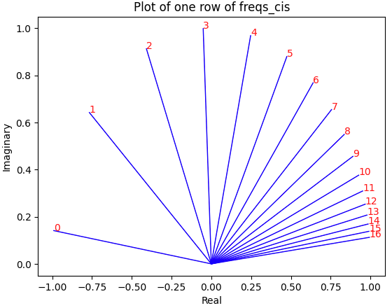
将频率转换为复数形式:
1 2 3 freqs_for_each_token = torch.outer(torch.arange(17 ), freqs)
torch.Size([17, 64])
绘制第 3 个 token 位置对应的前 17 个频率分量的复数表示:
1 2 3 4 5 6 7 8 9 value = freqs_cis[3 ]for i, element in enumerate (value[:17 ]):0 , element.real], [0 , element.imag], color='blue' , linewidth=1 , label=f"Index: {i} " )f"{i} " , xy=(element.real, element.imag), color='red' )'Real' )'Imaginary' )'Plot of one row of freqs_cis' )
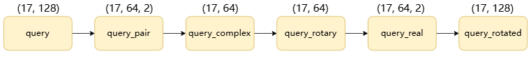
4.1.5 query_rotated
针对每个 token,将 128 个长度的 query 分为 64 对:
1 2 q_per_token_split_into_pairs = q_per_token.float ().view(q_per_token.shape[0 ], -1 , 2 )
torch.Size([17, 64, 2])
将 query 对转换为 query 复数:
1 2 q_per_token_as_complex_numbers = torch.view_as_complex(q_per_token_split_into_pairs)
torch.Size([17, 64])
进行点积以根据位置旋转 query 复数,每一个都旋转 $m*\theta$,$m$ 是旋转 query 的 token 的位置:
1 2 q_per_token_as_complex_numbers_rotated = q_per_token_as_complex_numbers * freqs_cis
torch.Size([17, 64])
将旋转的 query 复数看作实数来返回旋转的 query 对:
1 2 q_per_token_split_into_pairs_rotated = torch.view_as_real(q_per_token_as_complex_numbers_rotated)
torch.Size([17, 64, 2])
将旋转的 query 对变成旋转的 query:
1 2 q_per_token_rotated = q_per_token_split_into_pairs_rotated.view(q_per_token.shape)
torch.Size([17, 128])
4.1.6 key_rotated
针对每个 token,将 128 个长度的 key 分为 64 对:
1 2 k_per_token_split_into_pairs = k_per_token.float ().view(k_per_token.shape[0 ], -1 , 2 )
torch.Size([17, 64, 2])
将 key 对转换为 key 复数:
1 2 k_per_token_as_complex_numbers = torch.view_as_complex(k_per_token_split_into_pairs)
torch.Size([17, 64])
进行点积以根据位置旋转 key 复数,每一个都旋转 $m*\theta$,$m$ 是旋转 key 的 token 的位置。将旋转的 key 复数看作实数来返回旋转的 key 对:
1 2 k_per_token_split_into_pairs_rotated = torch.view_as_real(k_per_token_as_complex_numbers * freqs_cis)
torch.Size([17, 64, 2])
将旋转的 key 对变成旋转的 key:
1 2 k_per_token_rotated = k_per_token_split_into_pairs_rotated.view(k_per_token.shape)
torch.Size([17, 128])
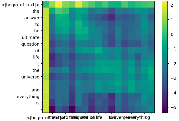
4.1.7 qk_score
将 query 和 key 相乘得到每个 token 相互映射的得分,表示每个 token 的 query 与每个 token 的 key 之间的相关度:
1 2 qk_per_token = torch.matmul(q_per_token_rotated, k_per_token_rotated.T)/(head_dim)**0.5
torch.Size([17, 17])
绘制 qk_score 矩阵的热力图:
1 2 3 4 5 6 7 8 9 10 def display_qk_heatmap (qk_per_token ):float ).detach(), cmap='viridis' )range (len (prompt_split_as_tokens)))range (len (prompt_split_as_tokens)))
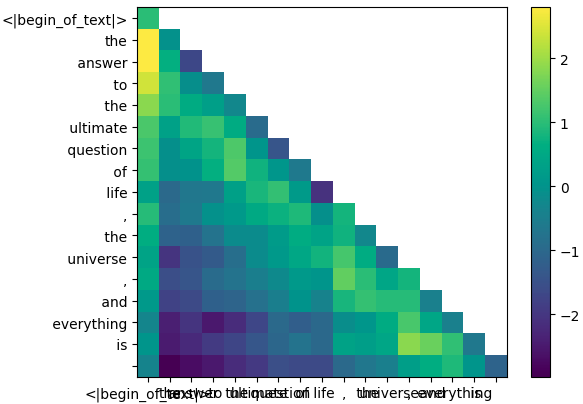
在 Llama3 的训练过程中,只学习使用过去的 token 来预测 token,因此将未来的 token 屏蔽为零。定义屏蔽矩阵:
1 2 3 mask = torch.full((len (tokens), len (tokens)), float ("-inf" ), device=tokens.device)1 )
tensor([[0., -inf, -inf, -inf, -inf, -inf, -inf, -inf, -inf, -inf, -inf, -inf, -inf, -inf, -inf, -inf, -inf],
[0., 0., -inf, -inf, -inf, -inf, -inf, -inf, -inf, -inf, -inf, -inf, -inf, -inf, -inf, -inf, -inf],
[0., 0., 0., -inf, -inf, -inf, -inf, -inf, -inf, -inf, -inf, -inf, -inf, -inf, -inf, -inf, -inf],
[0., 0., 0., 0., -inf, -inf, -inf, -inf, -inf, -inf, -inf, -inf, -inf, -inf, -inf, -inf, -inf],
[0., 0., 0., 0., 0., -inf, -inf, -inf, -inf, -inf, -inf, -inf, -inf, -inf, -inf, -inf, -inf],
[0., 0., 0., 0., 0., 0., -inf, -inf, -inf, -inf, -inf, -inf, -inf, -inf, -inf, -inf, -inf],
[0., 0., 0., 0., 0., 0., 0., -inf, -inf, -inf, -inf, -inf, -inf, -inf, -inf, -inf, -inf],
[0., 0., 0., 0., 0., 0., 0., 0., -inf, -inf, -inf, -inf, -inf, -inf, -inf, -inf, -inf],
[0., 0., 0., 0., 0., 0., 0., 0., 0., -inf, -inf, -inf, -inf, -inf, -inf, -inf, -inf],
[0., 0., 0., 0., 0., 0., 0., 0., 0., 0., -inf, -inf, -inf, -inf, -inf, -inf, -inf],
[0., 0., 0., 0., 0., 0., 0., 0., 0., 0., 0., -inf, -inf, -inf, -inf, -inf, -inf],
[0., 0., 0., 0., 0., 0., 0., 0., 0., 0., 0., 0., -inf, -inf, -inf, -inf, -inf],
[0., 0., 0., 0., 0., 0., 0., 0., 0., 0., 0., 0., 0., -inf, -inf, -inf, -inf],
[0., 0., 0., 0., 0., 0., 0., 0., 0., 0., 0., 0., 0., 0., -inf, -inf, -inf],
[0., 0., 0., 0., 0., 0., 0., 0., 0., 0., 0., 0., 0., 0., 0., -inf, -inf],
[0., 0., 0., 0., 0., 0., 0., 0., 0., 0., 0., 0., 0., 0., 0., 0., -inf],
[0., 0., 0., 0., 0., 0., 0., 0., 0., 0., 0., 0., 0., 0., 0., 0., 0.]])
绘制屏蔽后 qk_score 矩阵的热力图:
1 2 qk_per_token_after_masking = qk_per_token + mask
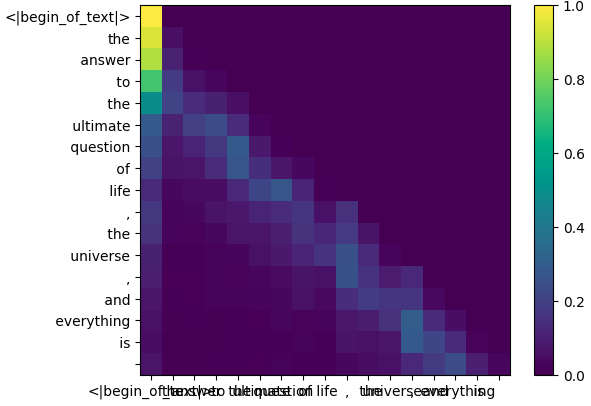
绘制 Softmax 后 qk_score 矩阵的热力图:
1 2 qk_per_token_after_masking_after_softmax = torch.nn.functional.softmax(qk_per_token_after_masking, dim=1 ).to(torch.bfloat16)
4.1.8 qkv_score qk_score 和每个 token 的 value 相乘后得到 qkv_score 矩阵:
1 2 qkv_attention = torch.matmul(qk_per_token_after_masking_after_softmax, v_per_token)
torch.Size([17, 128])
4.2 多头注意力
执行循环,来计算第一层中剩余 31 个注意力头的 qkv_score:
现实中每一层中的所有注意力头是并行计算的。
1 2 3 4 5 6 7 8 9 10 11 12 13 14 15 16 17 18 19 20 21 22 23 24 25 26 27 28 29 30 qkv_attention_store = []for head in range (n_heads):4 ]4 ]float ().view(q_per_token.shape[0 ], -1 , 2 )len (tokens)])float ().view(k_per_token.shape[0 ], -1 , 2 )len (tokens)])128 )**0.5 len (tokens), len (tokens)), float ("-inf" ), device=tokens.device)1 )1 ).to(torch.bfloat16)len (qkv_attention_store)
32
现在第一层上的所有 32 个头都有了 qkv_score,合并为一个大矩阵:
1 2 stacked_qkv_attention = torch.cat(qkv_attention_store, dim=-1 )
torch.Size([17, 4096])
4.3 output
查看第一层的 output 权重矩阵:
key 和 value 的维度被减小是为了减少计算复杂度和内存消耗,而保持 query 和 output 的较高维度是为了保留更多的信息。
1 2 w_layer0 = model["layers.0.attention.wo.weight" ]
torch.Size([4096, 4096])
将合并的大 qkv_score 矩阵和第一层的 output 权重矩阵进行矩阵乘法:
1 2 embedding_delta = torch.matmul(stacked_qkv_attention, w_layer0.T)
torch.Size([17, 4096])
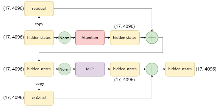
5 第一层 Layer 的剩余流程
进行残差连接:
1 2 embedding_after_edit = token_embeddings_unnormalized + embedding_delta
torch.Size([17, 4096])
进行归一化:
1 2 embedding_after_edit_normalized = rms_norm(embedding_after_edit, model["layers.0.ffn_norm.weight" ])
torch.Size([17, 4096])
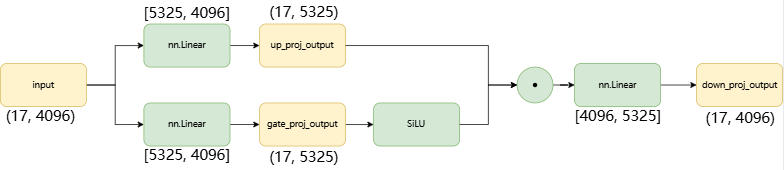
进行 MLP:
MLP 是一种特殊的 FFN,比传统 FFN 的维度小,利用率高。它引入了门控技术,gate_proj 为门控投影,up_proj 为升维投影,down 为降维投影,SiLU 用于门控过滤信息。
1 2 3 4 5 w1 = model["layers.0.feed_forward.w1.weight" ]"layers.0.feed_forward.w2.weight" ]"layers.0.feed_forward.w3.weight" ]
torch.Size([17, 4096])
进行残差连接:
1 2 layer_0_embedding = embedding_after_edit+output_after_feedforward
torch.Size([17, 4096])
6 升维和降维 升维通常是为了增加模型的容量,使其能够捕捉更复杂的特征和模式。当输入数据被映射到一个更高维度的空间时,不同的特征组合可以被模型更容易地区分。这在处理非线性问题时尤其有用,因为它可以帮助模型学习到更复杂的决策边界 。
降维则是为了减少模型的复杂性和过拟合的风险。通过减少特征空间的维度,模型可以被迫学习更加精炼和泛化的特征表示。此外,降维可以作为一种正则化手段,有助于提高模型的泛化能力。在某些情况下,降维还可以减少计算成本和提高模型的运行效率 。
在实际应用中,升维后再降维的策略可以被视为一种特征提取和变换的过程。在这个过程中,模型首先通过增加维度来探索数据的内在结构,然后通过降维来提取最有用的特征和模式。这种方法可以帮助模型在保持足够复杂性的同时,避免过度拟合训练数据 。
7 每层 layer 现在终于在第一层之后为每个 token 提供了新的 token embedding,之后的 31 层也是一样的处理过程:
1 2 3 4 5 6 7 8 9 10 11 12 13 14 15 16 17 18 19 20 21 22 23 24 25 26 27 28 29 30 31 32 33 34 35 36 37 38 39 40 41 42 43 44 45 46 47 48 49 50 51 final_embedding = token_embeddings_unnormalizedfor layer in range (n_layers):f"layers.{layer} .attention_norm.weight" ])f"layers.{layer} .attention.wq.weight" ]0 ] // n_heads, dim)f"layers.{layer} .attention.wk.weight" ]0 ] // n_kv_heads, dim)f"layers.{layer} .attention.wv.weight" ]0 ] // n_kv_heads, dim)f"layers.{layer} .attention.wo.weight" ]for head in range (n_heads):4 ]4 ]float ().view(q_per_token.shape[0 ], -1 , 2 )float ().view(k_per_token.shape[0 ], -1 , 2 )128 )**0.5 len (token_embeddings_unnormalized), len (token_embeddings_unnormalized)), float ("-inf" ))1 )1 ).to(torch.bfloat16)1 )f"layers.{layer} .attention.wo.weight" ]f"layers.{layer} .ffn_norm.weight" ])f"layers.{layer} .feed_forward.w1.weight" ]f"layers.{layer} .feed_forward.w2.weight" ]f"layers.{layer} .feed_forward.w3.weight" ]"norm.weight" ])1 ], model["output.weight" ].T)1 ], model["output.weight" ].T)print (f"输入 MLP:{tokenizer.decode([torch.argmax(before_mlp_logits, dim=-1 ).item()])} , 输出 MLP:{tokenizer.decode([torch.argmax(after_mlp_logits, dim=-1 ).item()])} " )
输入 MLP:ival, 输出 MLP:Disposition
输入 MLP:ौल, 输出 MLP:.updateDynamic
输入 MLP:opsy, 输出 MLP: Oaks
输入 MLP: Oaks, 输出 MLP:.stamp
输入 MLP:_stamp, 输出 MLP:RYPTO
输入 MLP:anker, 输出 MLP:ズ
输入 MLP:ズ, 输出 MLP:лишком
输入 MLP:BERS, 输出 MLP: nông
输入 MLP:ンチ, 输出 MLP:ilio
输入 MLP: Sez, 输出 MLP:tempts
输入 MLP:ilio, 输出 MLP:HAV
输入 MLP:HAV, 输出 MLP:ustum
输入 MLP: nebu, 输出 MLP:CRET
输入 MLP: Roose, 输出 MLP:\Dependency
输入 MLP:�, 输出 MLP:#af
输入 MLP:wang, 输出 MLP:iteDatabase
输入 MLP:SEX, 输出 MLP:'gc
输入 MLP:STRUCTIONS, 输出 MLP:ęk
输入 MLP:ęk, 输出 MLP:'gc
输入 MLP: answers, 输出 MLP: answer
输入 MLP: answer, 输出 MLP:рд
输入 MLP:рд, 输出 MLP:answered
输入 MLP:answered, 输出 MLP:answered
输入 MLP:answered, 输出 MLP:42
输入 MLP:42, 输出 MLP:42
输入 MLP:42, 输出 MLP:42
输入 MLP:42, 输出 MLP:42
输入 MLP:42, 输出 MLP:42
输入 MLP:42, 输出 MLP:42
输入 MLP:42, 输出 MLP:42
输入 MLP:42, 输出 MLP:42
输入 MLP:42, 输出 MLP:42
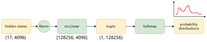
8 LogitLens
经过 32 层 Layers 后,得到了最终的 token embedding,对其进行归一化:
1 2 final_embedding = rms_norm(final_embedding, model["norm.weight" ])
torch.Size([17, 4096])
查看最后一个线性层的权重矩阵:
1 model["output.weight" ].shape
torch.Size([128256, 4096])
得到下一个预测的 token 的概率分布(通常还要对概率分布进行 Softmax):
模型中最后一个线性层的输出称为 logits,表示未缩放的“概率”,但总和不为1,因此需要 Softmax。只有最后一个 token embedding 用于预测
1 2 logits = torch.matmul(final_embedding[-1 ], model["output.weight" ].T)
torch.Size([128256])
取其概率最高的 token 作为预测结果:
1 2 next_token = torch.argmax(logits, dim=-1 )
tensor(2983)
对预测的 token 解码:
1 tokenizer.decode([next_token.item()])
'42'
9 采样策略
Greedy Search:每一步自回归都选择概率最高的 token。
Beam Search:保留固定束宽的候选序列,最终选择整体概率最高的序列。
Top-K:仅从概率最高的 K 个 token 中采样。
Top-P:动态选择累积概率超过 P 的最小 token 集合。
Random Sampling:按照概率分布随机采样。
Temperature:温度越高,概率分布越平缓,多样性越高;温度越低,概率分布越陡峭,风格越鲜明。